Notizblock

This is the english version. Bild

Eine deutschspachige Version findet sich hier
Bild

Index: constant force | constant coordinate acceleration | constant power, discussion (autotranslate from german): click here

CONSTANT FORCE

The velocity v is derived over the gammafactor γ

$Bild$

and the relativistic momentum p

$Bild$

where the force F, rest mass m and proper acceleration a

$Bild$

are connected with the differential of momentum p over coordinate time t. With that and F=constant we get

$Bild$

Plot with coordinate time t as x-axis (SI-units, momentum and energy as specific quantities per kg rest mass):

Bild

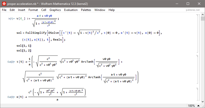
Analytical solutions for proper time τ and distance x:

Bild

Code:

Code: Alles auswählen

(* Eigenbeschleunigung, Methode 1 *) 

a=1000000m/sek^2;                                              (* Beschleunigung *) 
v0=0m/sek;                                             (* Anfangsgeschwindigkeit *) 

c=3*^8m/sek;                                             (* Lichtgeschwindigkeit *) 
m=sek=1;                                                            (* Einheiten *) 

γ[v_]:=1/Sqrt[1-v^2/c^2]; γ0=γ[v0];                                     (* Gamma *) 
v[t_]:=(a t+v0 γ0)/Sqrt[1+(a t+v0 γ0)^2/c^2];                 (* Geschwindigkeit *) 
e[t_]:=c^2 γ[v[t]]-c^2;                        (* spezifische kinetische Energie *) 
p[t_]:=v[t]γ[v[t]];                                       (* spezifischer Impuls *) 

sol=NDSolve[{τ'[t]==Sqrt[1-v[t]^2/c^2], τ[0]==0, X'[t]==v[t], X[0]==0}, 
{τ, X}, {t, 0, 1000}, Method->{"ImplicitRungeKutta", "DifferenceOrder"->20}, 
MaxSteps->Infinity, InterpolationOrder->All, WorkingPrecision->32]; 

т[t_]:=Evaluate[τ[t]/.sol][[1]];                                    (* Eigenzeit *) 
ť[t_]:=т'[t]; ṫ[t_]:=1/ ť[t];                                  (* Zeitdilatation *) 
α[t_]:=Evaluate[X''[t]/.sol][[1]];                  (* Koordinatenbeschleunigung *) 
A[t_]:=α[t] γ[v[t]]^3;                                    (* Eigenbeschleunigung *) 
x[t_]:=Evaluate[X[t]/.sol][[1]];                                     (* Position *) 

plot[f_]:=Plot[f[t], {t, 0, 1000}, Frame->True, ImagePadding->{{50, 8}, {16, 8}}, 
ImageSize->320, PlotRange->All, PlotStyle->Thick, AspectRatio->1/2] 

Grid[{{plot[т], plot[ť]}, 
{"      Eigenzeit τ", "      Zeitdilatation dτ/dt"}, 
{}, {plot[v], plot[p]}, 
{"      Geschwindigkeit v", "      Impuls p"}, 
{}, {plot[x], plot[e]}, 
{"      Strecke x", "      kinetische Energie"}, 
{}, {plot[A], plot[α]}, 
{"      Eigenbeschleunigung a", "      Koordinatenbeschleunigung α"}}, 
Alignment->Center]

Code: Alles auswählen

(* Eigenbeschleunigung, Methode 2 *) 

a=1000000m/sek^2;                                              (* Beschleunigung *) 
v0=0m/sek;                                             (* Anfangsgeschwindigkeit *) 

c=3*^8m/sek;                                             (* Lichtgeschwindigkeit *) 
m=sek=1;                                                            (* Einheiten *)

γ[v_]:=1/Sqrt[1-v^2/c^2]; γ0=γ[v0];                                     (* Gamma *) 
e[t_]:=c^2 γ[v[t]]-c^2;                        (* spezifische kinetische Energie *) 
p[t_]:=v[t] γ[v[t]];                                      (* spezifischer Impuls *) 

sol=NDSolve[{τ'[t]==Sqrt[1-V[t]^2/c^2], τ[0]==0, 
(V[t]^2 V'[t])/(c^2 (1-V[t]^2/c^2)^(3/2))+V'[t]/Sqrt[1-V[t]^2/c^2]==a, V[0]==v0, 
X'[t]==V[t], X[0]==0}, {τ, V, X}, {t, 0, 1000}, 
Method->{"ImplicitRungeKutta", "DifferenceOrder"->20}, MaxSteps->Infinity, 
InterpolationOrder->All, WorkingPrecision->32]; 

т[t_]:=Evaluate[τ[t]/.sol][[1]];                                    (* Eigenzeit *) 
v[t_]:=Evaluate[V[t]/.sol][[1]];                              (* Geschwindigkeit *) 
ť[t_]:=т'[t]; ṫ[t_]:=1/ť[t]                                    (* Zeitdilatation *) 
α[t_]:=Evaluate[X''[t]/.sol][[1]];                  (* Koordinatenbeschleunigung *) 
A[t_]:=α[t]γ[v[t]]^3;                                     (* Eigenbeschleunigung *) 
x[t_]:=Evaluate[X[t]/.sol][[1]];                                     (* Position *) 

plot[f_]:=Plot[f[t], {t, 0, 1000}, Frame->True, ImagePadding->{{50, 8}, {16, 8}}, 
ImageSize->320, PlotRange->All, PlotStyle->Thick, AspectRatio->1/2] 

Grid[{{plot[т], plot[ť]}, 
{"      Eigenzeit τ", "      Zeitdilatation dτ/dt"}, 
{}, {plot[v], plot[p]}, 
{"      Geschwindigkeit v", "      Impuls p"}, 
{}, {plot[x], plot[e]}, 
{"      Strecke x", "      kinetische Energie"}, 
{}, {plot[A], plot[α]}, 
{"      Eigenbeschleunigung a", "      Koordinatenbeschleunigung α"}}, 
Alignment->Center]

Code: Alles auswählen

(* Eigenbeschleunigung, Methode 3 *) 

a=1000000m/sek^2;                                              (* Beschleunigung *) 
v0=0m/sek;                                             (* Anfangsgeschwindigkeit *) 

c=3*^8m/sek;                                             (* Lichtgeschwindigkeit *) 
m=sek=1;                                                            (* Einheiten *) 

γ[v_]:=1/Sqrt[1-v^2/c^2]; γ0=γ[v0];                                     (* Gamma *) 
e[t_]:=c^2 γ[v[t]]-c^2;                        (* spezifische kinetische Energie *) 
p[t_]:=v[t] γ[v[t]];                                      (* spezifischer Impuls *) 
sol=NDSolve[{T'[τ]==1/Sqrt[1-V[τ]^2/c^2], T[0]==0, V'[τ]==a(1-V[τ]^2/c^2), 
V[0]==v0, X'[τ]==V[τ]/Sqrt[1-V[τ]^2/c^2], X[0]==0}, {V, T, X}, {τ, 0, 1000}, 
Method->{"ImplicitRungeKutta", "DifferenceOrder"->20}, MaxSteps->Infinity, 
InterpolationOrder->All, WorkingPrecision->32]; 

t[τ_]:=Evaluate[T[τ]/.sol][[1]];                              (* Koordinatenzeit *) 
т=Interpolation[Table[{t[j], j}, {j, 0, 1000}]];                    (* Eigenzeit *) 
v[t_]:=Evaluate[V[т[t]]/.sol];                                (* Geschwindigkeit *) 
ṫ[t_]:=Evaluate[T'[т[t]]/.sol]; ť[t_]:=1/ṫ[t];                 (* Zeitdilatation *) 
α[t_]:=x''[t];                                      (* Koordinatenbeschleunigung *) 
A[t_]:=α[t]γ[v[t]]^3;                                     (* Eigenbeschleunigung *) 
x[t_]:=Evaluate[X[т[t]]/.sol];                                       (* Position *) 

plot[f_]:=Plot[f[t], {t, 0, 1000}, Frame->True, ImagePadding->{{50, 8}, {16, 8}}, 
ImageSize->320, PlotRange->All, PlotStyle->Thick, AspectRatio->1/2] 

Grid[{{plot[т], plot[ť]}, 
{"      Eigenzeit τ", "      Zeitdilatation dτ/dt"}, 
{}, {plot[v], plot[p]}, 
{"      Geschwindigkeit v", "      Impuls p"}, 
{}, {plot[x], plot[e]}, 
{"      Strecke x", "      kinetische Energie"}, 
{}, {plot[A], plot[α]}, 
{"      Eigenbeschleunigung a", "      Koordinatenbeschleunigung α"}}, 
Alignment->Center]

For a side by side comparison of the 3 different ways to do it click here

CONSTANT COORDINATE ACCELERATION

With α=dv/dt=d²x/dt²=a/γ³=constant the equation for v is simply

$Bild$

With constant coordinate acceleration the speed of light would be reached when

$Bild$

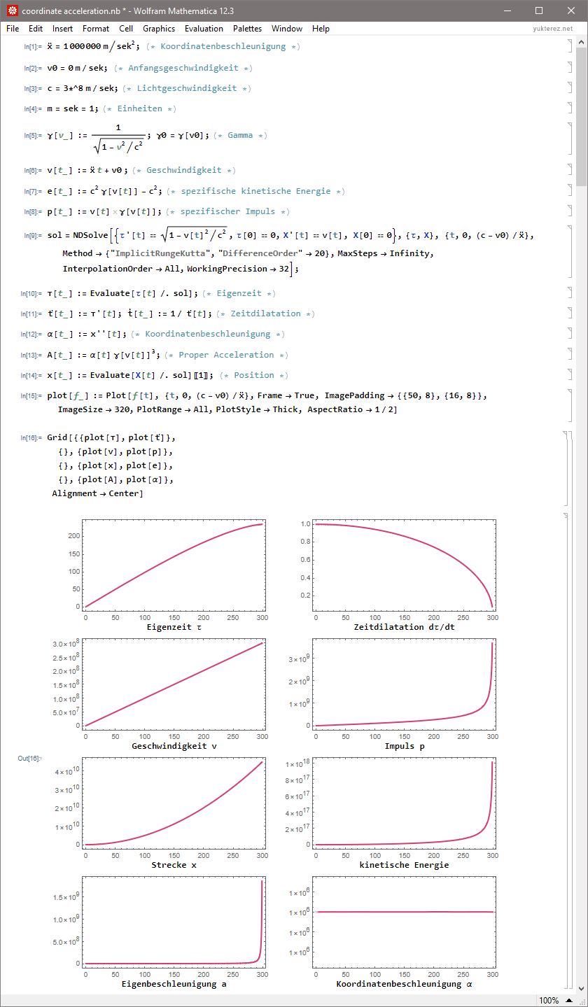
Plot with coordinate time t as x-axis (SI-units, momentum and energy as specific quantities per kg rest mass):

Bild

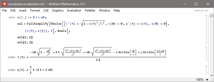
Analytical solutions for proper time τ and distance x:

Bild

Code:

Code: Alles auswählen

(* konstante Koordinatenbeschleunigung ẍ *) 

ẍ=1000000m/sek^2;                                   (* Koordinatenbeschleunigung *) 
v0=0m/sek;                                             (* Anfangsgeschwindigkeit *) 

c=3*^8m/sek;                                             (* Lichtgeschwindigkeit *) 
m=sek=1;                                                            (* Einheiten *) 

γ[v_]:=1/Sqrt[1-v^2/c^2]; γ0=γ[v0];                                     (* Gamma *) 
v[t_]:=ẍ t+v0 ;                                               (* Geschwindigkeit *) 
e[t_]:=c^2 γ[v[t]]-c^2;                        (* spezifische kinetische Energie *) 
p[t_]:=v[t]γ[v[t]];                                       (* spezifischer Impuls *) 

sol=NDSolve[{τ'[t]==Sqrt[1-v[t]^2/c^2], τ[0]==0, X'[t]==v[t], X[0]==0}, 
{τ, X}, {t, 0, (c-v0)/ẍ-1}, 
Method->{"ImplicitRungeKutta", "DifferenceOrder"->20}, 
MaxSteps->Infinity, InterpolationOrder->All, WorkingPrecision->32]; 

т[t_]:=Evaluate[τ[t]/.sol];                                         (* Eigenzeit *) 
ť[t_]:=т'[t]; ṫ[t_]:=1/ ť[t];                                  (* Zeitdilatation *) 
α[t_]:=x''[t];                                      (* Koordinatenbeschleunigung *) 
A[t_]:=α[t] γ[v[t]]^3;                                    (* Eigenbeschleunigung *) 
x[t_]:=Evaluate[X[t]/.sol][[1]];                                     (* Position *) 

plot[f_]:=Plot[f[t], {t, 0, (c-v0)/ẍ-1}, 
Frame->True, ImagePadding->{{50, 8}, {16, 8}}, ImageSize->320, 
PlotRange->All, PlotStyle->Thick, AspectRatio->1/2]

Grid[{{plot[т], plot[ť]}, 
{"      Eigenzeit τ", "      Zeitdilatation dτ/dt"}, 
{}, {plot[v], plot[p]}, 
{"      Geschwindigkeit v", "      Impuls p"}, 
{}, {plot[x], plot[e]}, 
{"      Strecke x", "      kinetische Energie"}, 
{}, {plot[A], plot[α]}, 
{"      Eigenbeschleunigung a", "      Koordinatenbeschleunigung α"}}, 
Alignment->Center]

CONSTANT POWER

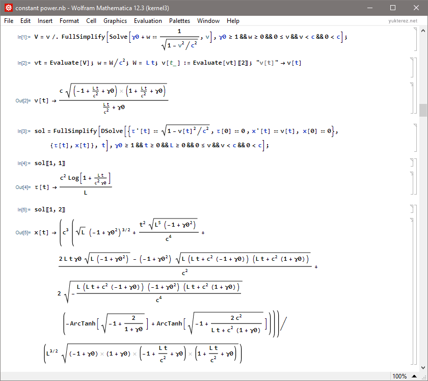
With constant power L the energy mc²γ inreases linearly with t. The initial energy plus the applied work equals the new energy

$Bild$

where W is the applied work

$Bild$

If we solve for v we get

$Bild$

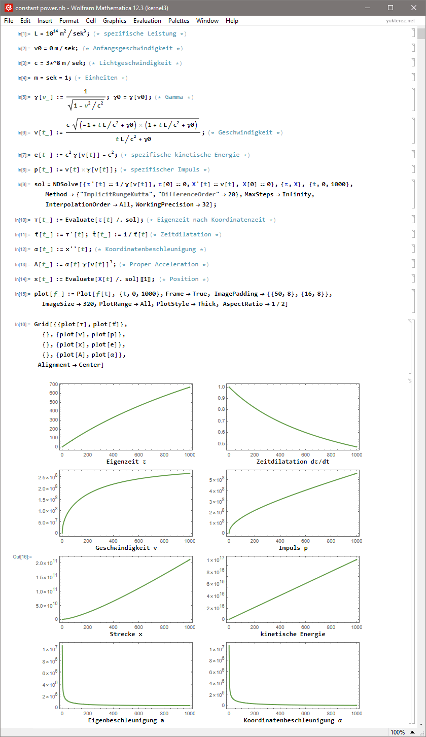
Plot with coordinate time t as x-axis (SI-units, momentum and energy as specific quantities per kg rest mass):

Bild

Analytical solutions for proper time τ and distance x:

Bild

Code:

Code: Alles auswählen

(* konstante Leistung *) 

L=10^14 m^2/sek^3;                                       (* spezifische Leistung *) 
v0=0m/sek;                                             (* Anfangsgeschwindigkeit *) 

c=3*^8m/sek;                                             (* Lichtgeschwindigkeit *) 
m=sek=1;                                                            (* Einheiten *) 

γ[v_]:=1/Sqrt[1-v^2/c^2]; γ0=γ[v0];                                     (* Gamma *) 
v[t_]:=(c Sqrt[(-1+t L/c^2+γ0) (1+t L/c^2+γ0)])/(t L/c^2+γ0); (* Geschwindigkeit *) 
e[t_]:=c^2 γ[v[t]]-c^2;                        (* spezifische kinetische Energie *) 
p[t_]:=v[t] γ[v[t]];                                      (* spezifischer Impuls *) 

sol=NDSolve[{τ'[t]==1/γ[v[t]], τ[0]==0, X'[t]==v[t], X[0]==0}, {τ, X}, 
{t, 0, 1000}, Method->{"ImplicitRungeKutta", "DifferenceOrder"->20}, 
MaxSteps->Infinity, InterpolationOrder->All, WorkingPrecision->32];

т[t_]:=Evaluate[τ[t]/.sol];                                         (* Eigenzeit *) 
ť[t_]:=т'[t]; ṫ[t_]:=1/ť[t];                                   (* Zeitdilatation *) 
x[t_]:=Evaluate[X[t]/.sol][[1]];                                     (* Position *) 
α[t_]:=Evaluate[X''[t]/.sol][[1]];                  (* Koordinatenbeschleunigung *) 
A[t_]:=α[t] γ[v[t]]^3;                                    (* Eigenbeschleunigung *) 

plot[f_]:=Plot[f[t], {t, 0, 1000}, 
Frame->True, ImagePadding->{{50, 8}, {16, 8}}, ImageSize->320, PlotRange->All, 
PlotStyle->Thick, AspectRatio->1/2]

Grid[{{plot[т], plot[ť]}, 
{"      Eigenzeit τ", "      Zeitdilatation dτ/dt"}, 
{}, {plot[v], plot[p]}, 
{"      Geschwindigkeit v", "      Impuls p"}, 
{}, {plot[x], plot[e]}, 
{"      Strecke x", "      kinetische Energie"}, 
{}, {plot[A], plot[α]}, 
{"      Eigenbeschleunigung a", "      Koordinatenbeschleunigung α"}}, 
Alignment->Center]

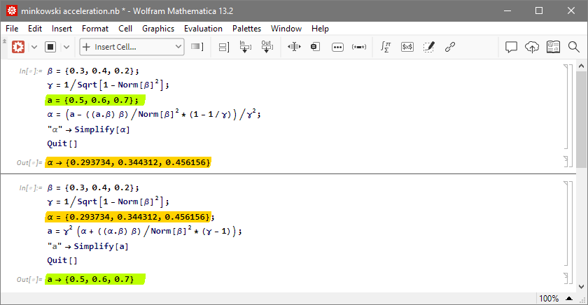
Vector notation: α is the coordinate acceleration of the accelerated observer in the unaccelerated frame, a is the proper acceleration of the accelerated observer in his own frame, v=βc is their relative velocity at the moment when they fly past each other:

$Bild$

Code:

Application in the context of the Schwarzschild metric: physics.stackexchange.com/a/842494

Notizblock

Relativistic Acceleration

Relativistic Acceleration

Relativistic Acceleration

Relativistic Acceleration

Relativistic Acceleration

Relativistic Acceleration